Which fields drive the h-index?
| Published |
| September 16, 2024 |
| Title |
| Which fields drive the h-index? |
| Authors |
| Paolo Giudici, Luca Boscolo. |
| DOI |
| 10.62684/FSOZ4761 |
| Keywords |
| H-index, Poisson models, Scaling |
Paolo Giudici(a), Luca Boscolo(b).
(a) Department of Economics and Management Sciences, University of Pavia, Italy.
(b) Top Italian Scientists founder.
Abstract
The measurement of the quality of academic research is often done by means of the h-index measure. Although widely accepted, the h-index has some issues and, in particular, it may depend on the scientific field in which a researcher operates. To date there is not a definitive answer as to whether this difference holds, and to what extent it varies. To fill the gap, we propose to operationally measure the difference in h-index across the sectors of a relatively homogeneous population of all scientists of a nation. To answer the heterogeneity issue we apply three different explainable machine learning models: linear regression, Poisson regression and tree models. Our results show that the latter two models better explain the data. They show that the only sectors for which a difference in h-index is significant are Physics, Biology and Clinical Sciences.
Introduction
The measurement of the quality of academic research is a rather controversial issue. in the 2000s [11] has proposed a measure that has the advantage of summarizing in a single summary statistics the information that is contained in the citation counts of each author. From that seminal paper, a large amount of research has been produces, focusing on in particular on the development of correction factors to the h index ([13], [3], [9]), [2], [12] that may take into account differences between sectors.
In this stream of research, [9] analysed the mathematical properties of the h index, and [3]proposed to employ a stochastic model for an author’s production/citation patterns. Following this mathematical formalisation, it becomes possible to analyse the h-index of individual researchers, whether or not in different fields, and compare them with each other.
Along a more empirical research line, [13] proposed to use a simple multiplicative correction to the h index to take into account the differences among researchers coming from different sectors, thus allowing a fair and sustainable comparison. They propose in particular a table with such normalizing factors, according to specific distributional assumptions of the citations. Their approach provides a simple way to explain and measure differences between different scientific fields. In a similar vein, [2] propose a rescaling procedure based on the Gini entropy and [12] propose a different rescaling, that takes into account the number of coautors: the fractional h-index.
We employ both streams of research as a starting point. More precisely, we follow [6], who, expanding the contribution of [9], propose a statistical approach that indicates that a Poisson distribution is a well suited approximation for the distribution of the h-index. In this paper we will show that a Poisson distribution is well suited to explain the drivers of the h-index. And we will employ this theoretical result to understand whether the h-index of a scientist depends on his/her filed of research, following the research line of [13], also followed by [15].
The paper is organized as follows: in Methodology section we review the proposal of [6] and formalise the model; in Application section we apply the new approach to a database of scientists homogeneous by nationality and, therefore, by scientific culture. Finally, Discussion section contains some concluding remarks.
Methodology
The paper of [11] has proposed a ”transparent, unbiased and very hard to rig measure” ([1]): the h index.
According to the definition, a scientist has index h if [math]\displaystyle{ h }[/math] of his or her n papers have at least [math]\displaystyle{ h }[/math] citations each and the other [math]\displaystyle{ (n-h) }[/math] papers have [math]\displaystyle{ ≤ h }[/math] citations each.
Following the work of Hirsch, many papers have discussed its application, especially in the bibliometric community. Some papers have focused on the statistical learning aspects behind the h index, and, among them, [9] who has stressed relevance of a ”statistical background” for the h index. Recently [?] has provided a complete statistical framework for the h index that holds for all sample sizes and respects the discrete nature of the citations data which are behind the h-index. We now recall their proposal as it dorms the basis of our analysis.
Let [math]\displaystyle{ X_1, . . . , X_n }[/math] be random variables which describe the number of citations of the n articles of a scientist. We assume that [math]\displaystyle{ X_1, . . . , X_n }[/math] are independent with a common citation distribution function [math]\displaystyle{ F }[/math]. Let us then assume that [math]\displaystyle{ F }[/math] is continuous, at least asymptotically, although the citation counts are integers. According to this assumption, the h index can be formally defined by the following:
| [math]\displaystyle{ h = 1 - F(h) = \frac{h}{n} }[/math] |
Then, following [6], assume that [math]\displaystyle{ F }[/math] is discrete. Given a set of n papers of a scientist to which a citations count vector [math]\displaystyle{ \underline{X} }[/math] is associated, consider the ordered sample of citations [math]\displaystyle{ {X_{(i)}} }[/math], that is [math]\displaystyle{ X_{(1)} ≥ X_{(2)} ≥ . . . ≥ X_{(n)} }[/math], from which obviously [math]\displaystyle{ X_{(1)} (X_{(n)}) }[/math] denotes the most (the least) cited paper. The h index can be defined as follows:
| [math]\displaystyle{ h = max(t : X_{(t)} ≥ t) }[/math] |
The distribution of the h index can then be shown to be:
| [math]\displaystyle{ p(h) = [F(X_{j(h)}) − F(X_{j(h)+1})]^{(n+1−h)} }[/math] |
The previous expression, albeit elegant, is non parametric, and is not so transparent in the estimation process.
To formulate a more explainable parametric specification, [6] suggested to follow the Loss Distribution Approach (LDA) employed in operational risk modelling (see [7] and [8]) where the losses are categorized in terms of ’frequency’ and ’severity’ (or impact). The frequency is the random number of loss events occurred during a specific time frame, while the severity is the mean impact of all such events in terms of monetary losses.
In the context of the h-index, the frequency is the (random) number of published papers along the career of a scientist and the impact is the (random) mean number of citations received in the same time frame by all such papers.
Let [math]\displaystyle{ Xi = (X_{i1}, X_{i2}, . . . , X_{ini}) }[/math] be a random vector containing the citations of the [math]\displaystyle{ n_i }[/math] papers published by the [math]\displaystyle{ i-th }[/math] scientist.
It follows that the total impact of a scientist [math]\displaystyle{ i }[/math] can be defined as the sum of a random number [math]\displaystyle{ n_i }[/math] of random citations:
| [math]\displaystyle{ Ci = X_{i1} + X_{i2} + . . . + X_{ini} }[/math] |
It can be shown that the above formula can be equivalently expressed as follows:
| [math]\displaystyle{ C_i = n_i × m_i }[/math] | (1) |
where [math]\displaystyle{ m_i = \frac{\sum_{j=1}^{n_i} X_{ij}}{n_i} }[/math] is the mean impact of a scientist.
Assuming that the scientists [math]\displaystyle{ i = 1, . . . , I }[/math] belong to a homogeneous community, conditionally on the production of each scientist (with number of papers equal to [math]\displaystyle{ n_i }[/math]), the citations of the papers [math]\displaystyle{ X_{ij} }[/math] , for [math]\displaystyle{ j = 1, . . . , n_i }[/math] are independent and identically distributed random variables, with common distribution [math]\displaystyle{ k(m_i) }[/math]:
| [math]\displaystyle{ k(x_{i1}) = k(x_{i2}) = . . . = k(x_{{in}_i}) = k(m_i) }[/math] |
[6] showed that, for each scientist [math]\displaystyle{ i }[/math], the distribution function of [math]\displaystyle{ C_i }[/math], that is [math]\displaystyle{ F(c_i) = P(C_i ≤ c_i) }[/math], can thus be found by means of a convolution between the distributions of [math]\displaystyle{ n_i }[/math] and [math]\displaystyle{ m_i }[/math] as follows:
| [math]\displaystyle{ F(c_i) = \sum_{n_i=1}^{\infty} p(n_i)k^{ni∗}(m_i) }[/math] |
where [math]\displaystyle{ c_i = n_i \times m_i }[/math] and [math]\displaystyle{ k^{ni∗} }[/math] indicates the n_i-fold convolution operator of the distribution [math]\displaystyle{ k(.) }[/math] with itself (see e.g. [4] and [?]):
| [math]\displaystyle{ k^{1∗}(mi) = k(m_i) }[/math] |
| [math]\displaystyle{ k^{n∗}(m_i) = k^{(n−1)∗}(m_i) ∗ k(m_i) }[/math] |
and, for each scientist, [math]\displaystyle{ p(n_i) }[/math] is the distribution of the number of produced papers and [math]\displaystyle{ k(m_i) }[/math] is the distribution of the mean impact.
In practice, the distribution functions [math]\displaystyle{ p(n_i) }[/math] and [math]\displaystyle{ k(m_i) }[/math] depend on unknown parameters, say [math]\displaystyle{ \lambda_i }[/math] and [math]\displaystyle{ θ_i }[/math]. A reasonable modeling assumption is that [math]\displaystyle{ n_i }[/math] , the number of published papers of a scientist in a specific community, follows a distribution [math]\displaystyle{ p(n_i|λ_i) }[/math] with [math]\displaystyle{ λ_i }[/math] a parameter that summarizes the productivity of each scientist and that, conditionally on [math]\displaystyle{ n_i }[/math], the paper citations [math]\displaystyle{ x_i }[/math] follows a distribution [math]\displaystyle{ k(m_i|θ_i, n_i) }[/math] with [math]\displaystyle{ θi }[/math] a parameter that is function of the mean impact that may vary across scientists.
To complete the proposed model, [6] showed that a reasonable starting assumption may be to take:
| [math]\displaystyle{ p(n_i|λ_i) ∼ Poisson(λ_i) }[/math] |
| [math]\displaystyle{ k(m_i|θ_i, n_i) ∼ Poisson(θ_i) }[/math] |
where [math]\displaystyle{ λ_i }[/math] and [math]\displaystyle{ θ_i }[/math] are unknown and strictly positive parameters to be estimated, representing, respectively, the mean number of published papers and the mean number of citations of each scientist (the mean impact).
The previous results implies that the statistical distribution of the h-index can be reasonably approximated by a Poisson distribution, assuming that the underlying population of scientists for which the h-index is calculated is homogeneous.
In the next section we will extend the literature aimed at comparing the h-index across different scientific fields employing a regression model based on the Poisson distribution and compare it with alternative machine learning formulations. the results obtained by employing the previous model.
Application
The Top Italian Scientists database started in 2010 when Luca Boscolo got inspired by an article that gathered a list of 300 Italian academics in Italy and abroad with the highest scientific impact in any area. To measure the scientific impact they used the h-index. Luca had the idea to download the entire list of the academics working for the Italian universities (about 54k people) and for each of them calculated their h-index using Google Scholar as database. Luca then extracted a list (about a 1k people) whose h-index was greater or equal than 30. The result was called “list Top Italian Scientists” (TIS), and a paper was published displaying a list of the Italian universities ordered by the number of TIS. The paper was cited by some of the main Italian newspapers such as La Stampa and it went viral scattering a huge interest in the academic world. After that, Luca started to get flooded with emails congratulating the work or indicating someone with h-index >= 30. After more than 12 years the list has grown up from a 1k to more than 5.5 k. Nowadays this list is known to all Italian academics working in Italy or abroad.
Note that this is indeed a small subset of the worldwide population of statisticians. However, these scientists forms a cohort of people that has grown their careers under similar conditions, especially in terms of common academic rules (they belong to the same country). To our knowledge this is the first time in bibliometric studies that a community of scientists belonging to the same country has been considered in the analysis.
We have extracted our data from the TIS list at 30 July 2023. For each scientist, we have been able to download its h-index, the total number of citations, and the scientific field of belonging. The following table presents, for each of the eleven considered fields, the number of top scientists contained in our sample: those with an h-index greater than 30 by 30 July, 2023.
| Macro | TIS | |
|---|---|---|
| 1 | MATHematics | 60 |
| 2 | COMPuter sciences | 208 |
| 3 | PHYSics | 643 |
| 4 | CHEMistry | 335 |
| 5 | NATUral sciences | 295 |
| 6 | BIOLogical sciences | 1133 |
| 7 | CLINical sciences | 917 |
| 8 | ENGIneering | 418 |
| 9 | HUMAnities | 3 |
| 10 | BUSIness sciences | 45 |
| 11 | SOCIal sciences | 11 |
Table 3 clearly shows that the number of top scientists is greatly unbalanced across the considered macroareas, which are those officially employed by Italian Universities, for teaching, funding and promotions, for example.
The previous figures should obviously be normalised by the total number of scientists present in each area, at the same day, which is contained in Table 3 below.
Dividing the counts in Table 3 by the total number of scientists in Table 3 we obtain the empirical probability that a scientist in a given scientific field (Macroarea) is included among Top Italian Scientists, having an h-index greater than 30. Such probabilities are reported in Table 3 below.
Table 3 indicates that the (estimated) probability that a scientists has an hindex greater than 30 is about 20% for researchers in Physics, Biological Sciences and Computer Science. It decreases below 10% for Chemistry and Clinical Sciences; around 5% for Natural Sciences and Engineering, and around 2% for Mathematics. Moving to socio-humanistic fields, the probability is around 0.78% for Business and Economics sciences, and 0.15% for the social sciences (which inbclude law and sociology). Finally, the same probability decreases to 0.3% for the humanities.
The above results are in line with the literature, and attribute the largest
| Macro | Total | |
|---|---|---|
| 1 | MATHematics | 2447 |
| 2 | COMPuter sciences | 1145 |
| 3 | PHYSics | 2788 |
| 4 | CHEMistry | 3320 |
| 5 | NATUral sciences | 4667 |
| 6 | BIOLogical sciences | 5464 |
| 7 | CLINical sciences | 10585 |
| 8 | ENGIneering | 11323 |
| 9 | HUMAnities | 9415 |
| 10 | BUSIness sciences | 5763 |
| 11 | SOCIal sciences | 7019 |
| Macro | Probabilities | |
|---|---|---|
| 1 | MATHematics | 0.0245 |
| 2 | COMPuter sciences | 0.1816 |
| 3 | PHYSics | 0.2306 |
| 4 | CHEMistry | 0.1009 |
| 5 | NATUral sciences | 0.0632 |
| 6 | BIOLogical sciences | 0.2073 |
| 7 | CLINical sciences | 0.0866 |
| 8 | ENGIneering | 0.0369 |
| 9 | HUMAnities | 0.0003 |
| 10 | BUSIness sciences | 0.0078 |
| 11 | SOCIal sciences | 0.0015 |
probability to the fields characterised by multiple autorships, such as Physics, Biological Sciences and Computer Science; differntly from fields such as Mathematics, Business Sciences or the Humanities.
A relatively lower value is received by Clinical Sciences and Engineering: with respect to these we recall that these fields are characterised by a large presence of professionals, who publish relatively less.
To better understand which fields drive higher h-indexes we now analyse the available dataset, composed of all italian scientists with h-index greater than 10, distributed by fileds as in 3. It is a population of 63396 scientists, with a total number of citations equal to 94890813: about 23326 per capita.
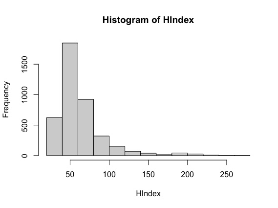
Figure 1 describes our data in terms of observed h-index for the overall population of scientists.
From Figure 3 note that the distribution of the h-index is, as expected, right skewed. The distribution of the citations, which we do not report for lack of space, look very similar. Indeed, the correlation coefficient between the h-index
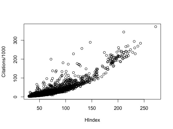
and the number of citations is equal to 0.904 as can be desumed from the observed scatterplot, reported in Figure 2 2 indicates the strong correlation between the h-index and the citations, which makes the two variables very similar to each other.
In Figure 3 we report the distribution of the h index by macroarea, by means of the conditional boxplots.
From Figure 3 note that Physics and Biological sciences show higher values (and more skewed distributions). Differently from what occurs in terms of the probability of becoming a top scientist, 3 shows a similar behaviour for Clinical Sciences, whereas Computer science is more similar to the other fields (and to Engineering in particular). These differences can be explained as follows. Professional clinical scientists, such as hospital doctors, lower the probability of becoming a top scientist; however, a clinical scientist that is a top scientist is mainly a researcher, typically with a large coautorship, like physicists and biologists. A similar behaviour, although to a more limited extent, occurs for engineers, business scientists and social scientists. The difference is more difficult to explain for computer scientists. One possible argument is that, because
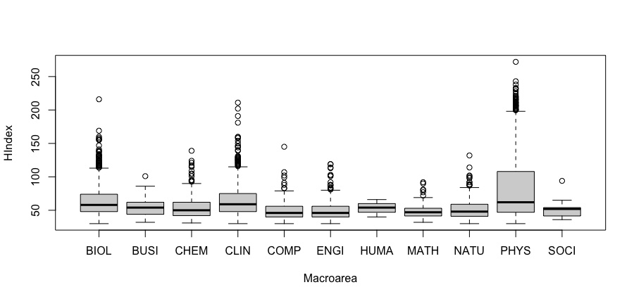
of multiple authorships, and the impact of their topic, relatively young scientists become soon top scientists, even with a limited number of papers. The h-index then takes longer to grow.
In this respect, the following Table 3 presents the correlation between hindex and the citations by field.
| Macro | cor | |
|---|---|---|
| 1 | BIOL | 0.83 |
| 2 | BUSI | 0.87 |
| 3 | CHEM | 0.65 |
| 4 | CLIN | 0.80 |
| 5 | COMP | 0.82 |
| 6 | ENGI | 0.87 |
| 7 | HUMA | 1.00 |
| 8 | MATH | 0.85 |
| 9 | NATU | 0.85 |
| 10 | PHYS | 0.96 |
| 11 | SOCI | 0.94 |
Indeed, 3 shows that correlations vary among sectors, and that Computer Science and Clinical Sciences have the lowest values, together with Chemistry, in line with our previous discussion.
We now more precisely measure the difference in h-indexes between the different fields, creating as many binary variables as are the scientific fields and applying a linear regression of the observed h-indexes with respect to such variables. To avoid perfect collinearity, the effect of the Humanities field is included in the intercept.
Table 3 present the results of the regression.
| Estimate | Std. Error | t value | [math]\displaystyle{ Pr(\gt |t|) }[/math] | |
|---|---|---|---|---|
| (Intercept) | 53.3333 | 16.3704 | 3.26 | 0.0011 |
| Biology | 10.2642 | 16.3921 | 0.63 | 0.5312 |
| Business | 1.2444 | 16.9073 | 0.07 | 0.9413 |
| Chemistry | 0.8607 | 16.4436 | 0.05 | 0.9583 |
| Clinical | 11.2043 | 16.3972 | 0.68 | 0.4945 |
| Computer | -3.7516 | 16.4881 | -0.23 | 0.8200 |
| Engineering | -3.2855 | 16.4291 | -0.20 | 0.8415 |
| Social | -1.0606 | 18.4683 | -0.06 | 0.9542 |
| Mathematics | -3.4000 | 16.7747 | -0.20 | 0.8394 |
| Natural | -1.8893 | 16.4535 | -0.11 | 0.9086 |
| Physics | 32.2561 | 16.4086 | 1.97 | 0.0494 |
Table 3 shows that only Physics has an h-index which significantly differs from the others.
However, consistently with the observed histogram, the distribution of the hindex is skewed and cannot be considered Gaussian. In line with what discussed in the methodological section, we can assume a Poisson distribution for the hindex and apply a generalised linear regression model with a Poisson link. Table 3 present the results of the Poisson regression.
| Estimate | Std. Error | t value | [math]\displaystyle{ Pr(\gt |t|) }[/math] | |
|---|---|---|---|---|
| (Intercept) | 3.9766 | 0.0791 | 50.30 | 0.0000 |
| Biology | 0.1760 | 0.0791 | 2.22 | 0.0262 |
| Business | 0.0231 | 0.0816 | 0.28 | 0.7774 |
| Chemistry | 0.0160 | 0.0794 | 0.20 | 0.8402 |
| Clinical | 0.1907 | 0.0792 | 2.41 | 0.0160 |
| Computer | -0.0729 | 0.0797 | -0.92 | 0.3599 |
| Engineering | -0.0636 | 0.0794 | -0.80 | 0.4230 |
| Social | -0.0201 | 0.0894 | -0.22 | 0.8222 |
| Mathematics | -0.0659 | 0.0811 | -0.81 | 0.4169 |
| Natural | -0.0361 | 0.0795 | -0.45 | 0.6500 |
| Physics | 0.4730 | 0.0792 | 5.97 | 0.0000 |
From table 3 note that, at a significance level of 5%, not only Physics, but also Biology and Clinical Sciences have an h-index which is significantly higher than for the other fields. This result is indeed more coherent with 3 than what obtained with the Guassian linear model in 3, bringing further evidence to the assumption of a Poisson distribution for the h-index.
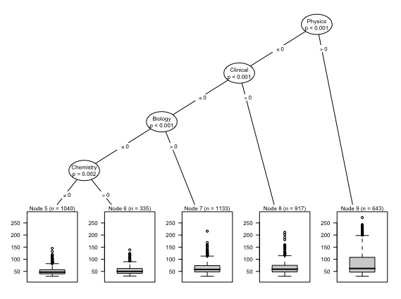
To robustify our results, we now consider the application of another explainable by design model, a regression tree.
Similarly to what done before, we consider the h-index as the response variable to be partitioned according to the found groupings of the binary variables that describe the scientific fields.
Figure 4 reports the results of the application of a regression tree model on the whole sample.
Figure 4 shows that Physics, Clinical Sciences, Biology, along with Chemistry, are the only relevant variables in the regression trees, in line with the results obtained with the Poisson regression. Evidently, the tree model, being non linear, can capture the deviation from the Gaussian distribution similarly to the Poisson regression.
Discussion
In this paper we have addressed the topic of comparing the h-index among different scientific fields.
To achieve this task, we have considered all the h-indexes of an homogeneous population, that of all italian researchers with an h-index greater than 30, acording to the information retrieved the Top Italian Scientists initiative. From a modelling viewpoint, we have compared alternative statistical and machine learning models. While the classical linear model is proved to be inadequate to model the h-index variable, both a Poisson regression and a non parametric tree model seem to give result consistent with the descriptive statistics, and the intuition.
Both Poisson regression and tree models are explainable, and both lead to the conclusion that the h-index of the researchers in Physics, Clinical Science and Biology are significantly higher than those of the scientists in other fields, which are instead similar to each other.
The above findings are complemented with a logistic regression model that explain the probability of becoming a top scientist, particularly useful for younger scientists. The results show that, besides researchers in Physics and Biology, also computer scientists have a higher chance of exceeding a large h-index (greater than 30).
More research is needed to further validate our results, possibly in different populations of scientists.
Declarations
Acknowledgment
The authors thank the Top Italian Scientists initiative for sharing the data.
Conflict of Interest
The Authors declare that there is no conflict of interest.
References
- Ball, P., Index aims for fair ranking of scientists, Nature, 436:900, (2005).
- Bir´o, T.S., Telcs, A., J´ozsa, M., N´eda,Z., Ball, P. Gintropic scaling of scientometric indexes. Physica A: Statistical Mechanics and its Applications, Volume 618, 2023.
- Burrell, Q. L., Hirsch’s h-index: A stochastic model, Journal of Informetrics, v. 1, p. 16-25, (2007).
- Buhlmann, H., Mathematical Methods in Risk Theory, Grundlehrenband 172, Springer-Verlag, Heidelberg, (1970).
- Cerchiello, P., and P. Giudici, On the distribution of functionals of discrete ordinal variables: Statistics & Probability Letters, v. 82, p. 2044-2049, 2012.
- Cerchiello, P., and P. Giudici, Cerchiello, P., Giudici, P. On a statistical H-index. Scientometrics, 99 pp. 299-312, 2013.
- Cruz M. G., ”Modeling, measuring and hedging operational risk.” Wiley (2002).
- Dalla Valle, L., and P. Giudici, A Bayesian approach to estimate the marginal loss distributions in operational risk management: Computational Statistics & Data Analysis, v. 52, p. 3107-3127, (2008).
- Glanzel, W., On the h-index - A mathematical approach to a new measure of publication activity and citation impact: Scientometrics, v. 67, p. 315-321, (2006).
- Harzing, A.W., Publish or Perish, available from http://www.harzing.com/pop.htm, (2007).
- Hirsch, J. E., An index to quantify an individual’s scientific research output: Proceedings of the National Academy of Sciences of the United States of America, v. 102, p. 16569-16572, (2005).
- Koltun, V., Hafner, D. The h-index is no longer an effective correlate of scientific reputation. Plos One (2021).
- Iglesias, J. E., and C. Pecharroman, Scaling the h-index for different scientific ISI fields: Scientometrics, v. 73, p. 303-320, (2007).
- Izsak, F., Maximum likelihood estimation for constrained parameters of multinomial distributions - Application to Zipf-Mandelbrot models: Computational Statistics & Data Analysis, v. 51, p. 1575-1583, (2006).
- Malesios, C.C., Psarakis, S Izsak, F. Comparison of the h-index for different fields of research using bootstrap methodology. Quality and Quantity 48, 521–545 (2014).
- Mandelbrot, B., On the theory of word frequencies and on related Markovian models of discourse. In R. Jakobson (ed.), Structure of Language and its Mathematical Aspects, pages 1909. American Mathematical Society, Providence, RI, (1962).
- Siegel, S., and Castellan, N.J., Nonparametric statistics for the behavioral sciences (2nd Ed.). New York, McGraw-Hill, (1988).
